

Using AI for Blockchain Data Analysis: A Beginner’s Guide with FRAX-WETH Price Prediction

Introduction
Hi, Dear Reader! This will be a simple demo of integrating AI into your blockchain project. By integrating AI into your blockchain project, you can unlock Pandora’s box to infinite potential. From something as simple as a smart price predictor (we will explore this today) to automated anomaly detection and beyond, every idea can be brought to life by using the right tools along with the right skills.
Project Scope
In this article, we will see how we can train a very simple AI model on public blockchain data to predict the price of FRAX tokens in terms of WETH tokens. Then we are also going to test our trained model on real-world data to check the accuracy of our model.
Due to the limited scope of this POC, I will be using a very simple AI model and not a NLP model. Because of this, the resulting accuracy may not be sufficient for your use case. Feel free to get in touch with us to know what fits your requirements.
Data Aggregator
Data aggregation plays the most important role when it comes to designing a prediction model based on blockchain data. A common approach can be to periodically run the model on the aggregated data. In the case of using a private blockchain, the data aggregation should be taken care of while deploying the blockchain. Since, in this POC, we will be constraining ourselves to the Ethereum blockchain, we will use Dune.com as our data aggregator.
Dune.com is a popular platform that lets you access various blockchain data and query it using SQL. Dune becomes the best choice of data aggregator because it provides the data in a structured format and hence we don’t have to worry about cleaning our data of unwanted records.
Follow the following steps to get started and run your first query:
- We start by signing up for Dune.com at their Sign Up Page.
- Click on the Create button on the top left corner and select New query.
- Next in the query window we use the following query:
          select
            block_time,
            blockchain,
            token_pair,
            token_bought_amount,
            token_bought_symbol,
            token_sold_amount,
            token_sold_symbol
          from dex.trades
          where
            token_pair = ‘FRAX-WETH’ and
            blockchain = ‘ethereum’
          order by block_time asc
Here, we are fetching the records from a table named dex.trades. This table keeps a record of all the trades taking place across multiple blockchains and different platforms. For now we are interested in only the FRAX-WETH pair in Ethereum and make use to query the necessary columns. We will sort our records in the ascending order of time since we want to train our model on the older data and then test our model on the latest 200 records.
- Click on the Run button to view the result of the query
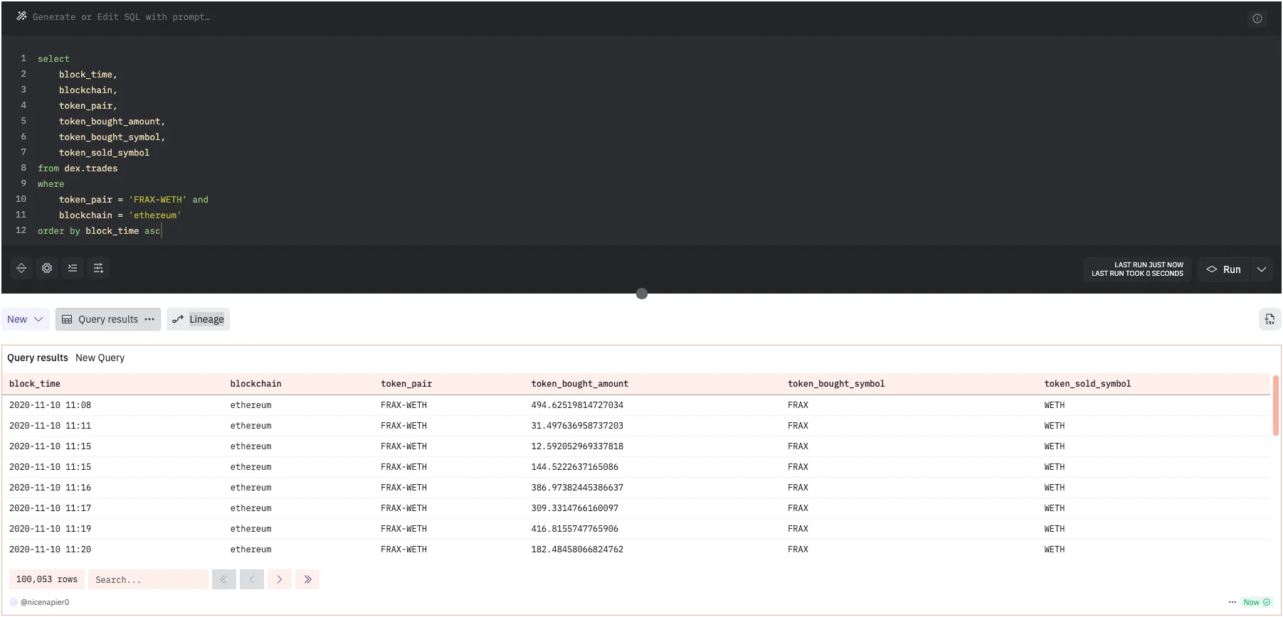
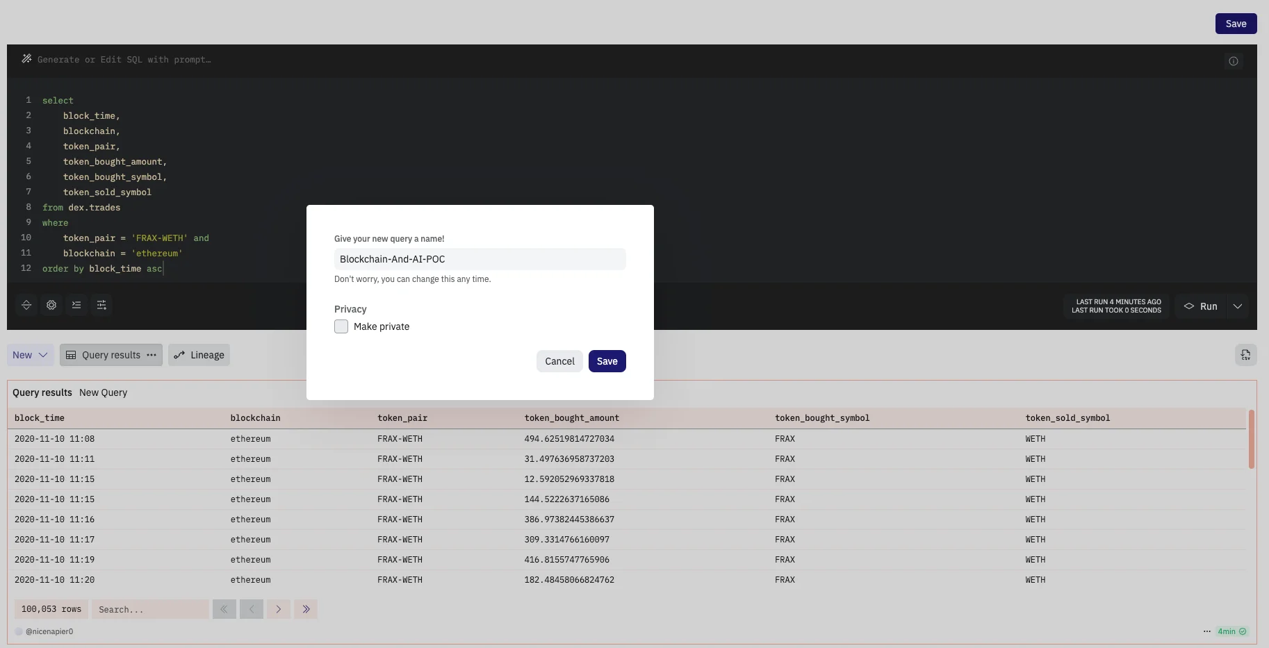
- Now click on the Save button to save this query. We have to save our query since we will be fetching this result from our script in the later part of this POC.
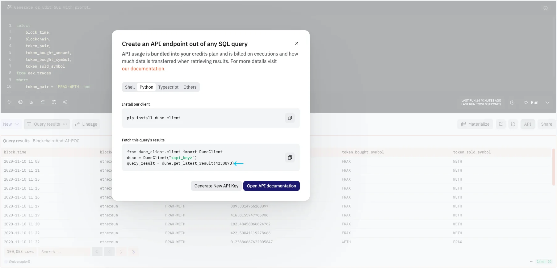
- By clicking on the API button we would be able to view the suggested code for accessing this data. Remember to take a node of the query id displayed in the suggested code
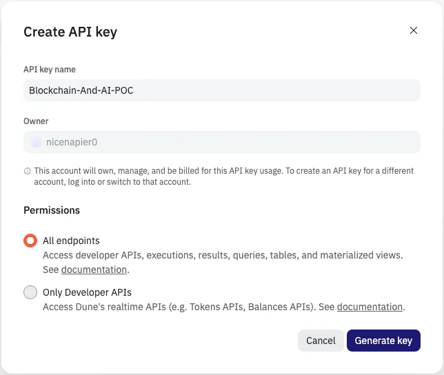
- The last step would be to create an API key. This API key will help us fetch our data through any Script for further processing. Head on to the Settings Page of Dune and generate new API key. Make sure to select All endpoints when generating the key
Now we are ready to develop our model using this data. In the next section we will discuss the steps to develop a simple AI model and predict future price.
Develop AI model
As you may have already expect, we will be using Python (inside a Jupyter Notebook) for developing our AI model. Before we can get started make with the code, make sure the following dependencies are installed:
- pandas ⇒ For processing the data.
- sklearn ⇒ For our AI models.
- xgboost ⇒ For metrics.
- dune_client ⇒ For fetching the query result from Dune.
- matplotlib ⇒ For plotting a graph visualising the end results.
Follow the following steps to develop, train and test your AI model:
- Set up a variable to store the API Key for Dune that we generated in the previous section.
API_KEY = “<YOUR API KEY>”
- Next we import all the required dependencies
          import pandas as pd
          from sklearn.model_selection import train_test_split, GridSearchCV
          from sklearn.metrics import mean_squared_error
          from xgboost import XGBRegressor
          from sklearn.ensemble import RandomForestRegressor, GradientBoostingRegressor, StackingRegressor
          from sklearn.linear_model import Ridge, Lasso
          from sklearn.preprocessing import MinMaxScaler

          import matplotlib.pyplot as plt
          import numpy as np
          from tqdm import tqdm
- Next we fetch the query result from Dune
          dune = DuneClient(API_KEY)
          query_result = dune.get_latest_result(4230873)
This will fetch the query result and load it in the query_result variable.
- Next we will store the data in a CSV file so that we don’t have to repeatedly fetch the data from Dune when we are working on different models. Use the following code to save the response in a CSV file
          data = query_result.result.rows
          df = pd.DataFrame(data)
          df.to_csv(‘dune_result.csv’, index=False)
- Use the following code to read the data from CSV file, define the model to be used and to train it.
          # Load the data
          df = pd.read_csv(‘dune_result.csv’)

          # Ensure the data is sorted in ascending order of block_time
          df = df.sort_values(by=’block_time’)

          # Calculate the price of FRAX in terms of WETH
          def calculate_price(row):
              if row[‘token_bought_symbol’] == ‘FRAX’ and row[‘token_sold_symbol’] == ‘WETH’:
                  if row[‘token_bought_amount’] > 0 and row[‘token_sold_amount’] > 0:
                      return row[‘token_bought_amount’] / row[‘token_sold_amount’
              elif row[‘token_sold_symbol’] == ‘FRAX’ and row[‘token_bought_symbol’] == ‘WETH’:
                  if row[‘token_sold_amount’] > 0 and row[‘token_bought_amount’] > 0:
                      return row[‘token_sold_amount’] / row[‘token_bought_amount’]
              return None
          df[‘price_frax_weth’] = df.apply(calculate_price, axis=1)

          # Drop rows with None values in ‘price_frax_weth’
          df = df.dropna(subset=[‘price_frax_weth’])

          # Feature engineering
          df[‘ratio_token_bought_sold’] = df[‘token_bought_amount’] / (df[‘token_sold_amount’] + 1e-9)
          df[‘day_of_week’] = pd.to_datetime(df[‘block_time’]).dt.dayofweek
          df[‘hour_of_day’] = pd.to_datetime(df[‘block_time’]).dt.hour

          # Scale the features
          scaler = MinMaxScaler()
          scaled_features = scaler.fit_transform(df[[‘token_bought_amount’, ‘token_sold_amount’, ‘ratio_token_bought_sold’, ‘day_of_week’, ‘hour_of_day’]])
          scaled_df = pd.DataFrame(scaled_features, columns=[‘token_bought_amount’, ‘token_sold_amount’, ‘ratio_token_bought_sold’, ‘day_of_week’, ‘hour_of_day’])
          X = scaled_df
          y = df[‘price_frax_weth’]

          # Split the data into oldest for training and latest 200 for testing
          X_train = X.iloc[:-500]
          y_train = y.iloc[:-500]
          X_test = X.iloc[-500:]
          y_test = y.iloc[-500:]
          print(len(X_train))
          print(len(X_test))

          # Define models
          models = {
              ‘XGBoost’: XGBRegressor(),
              ‘RandomForest’: RandomForestRegressor(),
              ‘GradientBoosting’: GradientBoostingRegressor(),
              ‘Ridge’: Ridge(),
              ‘Lasso’: Lasso()
          }

          # Hyperparameter tuning and training
          best_models = {}
          for name, model in tqdm(models.items(), desc=”Training Models”):
              if name in [‘XGBoost’, ‘RandomForest’, ‘GradientBoosting’]:
                  param_grid = {
                      ‘n_estimators’: [50, 100, 200],
                      ‘max_depth’: [3, 4, 5]
                  }
              elif name in [‘Ridge’, ‘Lasso’]:
                  param_grid = {
                      ‘alpha’: [0.01, 0.1, 1.0, 10.0]
                  }
              grid_search = GridSearchCV(model, param_grid, scoring=’neg_mean_squared_error’, cv=3, verbose=1)
              grid_search.fit(X_train, y_train)
              best_models[name] = grid_search.best_estimator_

          # Stacking ensemble for improved performance
          stacking_regressor = StackingRegressor(
              estimators=[(‘xgb’, best_models[‘XGBoost’]),
                          (‘rf’, best_models[‘RandomForest’]),
                          (‘gb’, best_models[‘GradientBoosting’])],
              final_estimator=Ridge()
          )
          stacking_regressor.fit(X_train, y_train)
          y_pred = stacking_regressor.predict(X_test)

          # Evaluate the model
          mse = mean_squared_error(y_test, y_pred)
          print(f”Mean Squared Error: {mse}”)

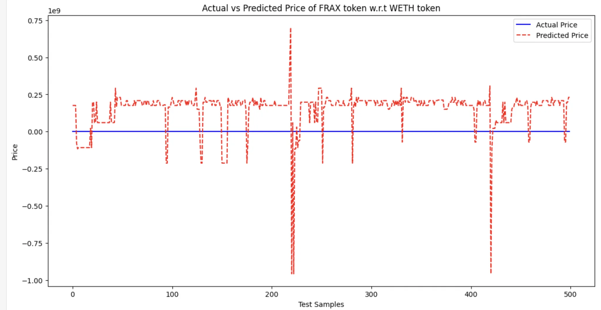
          # Plot the results
          plt.figure(figsize=(14, 7))
          plt.plot(y_test.values, color=’blue’, label=’Actual Price’)
          plt.plot(y_pred, color=’red’, linestyle=’dashed’, label=’Predicted Price’)
          plt.title(‘Actual vs Predicted Price of FRAX token w.r.t WETH token’)
          plt.xlabel(‘Test Samples’)
          plt.ylabel(‘Price’)
          plt.legend()
          plt.show()
- Once the processing is completed, you will get the prediction result in a graph format. It may look something like the following:
Conclusion
This blog shows how AI models can be integrated with AI. However the model is quite rudimentary for any production grade application. There are multiple deciding factors involved in the processing of using AI models to make predictions based on past data stored in the blockchain.
Interested in learning more about x-enabler?



Leave a comment!